Loss Crossovers and Phase Transitions Under Ambient Training in Diffusion Models
Abstract
The distinct behaviours of memorisation and generalisation in generative models has been noted empirically, and linked to sharp phase transitions as model capacity increases. Further, recent work has shown that for the standard diffusion loss objective crossovers between memorising and generalising solutions predict the phase transition location. We investigate how loss crossovers behave in the ambient regime introduced by Shah et al. (2025). Our main result in fig. 2, shows that crossover locations inherit the same bell-shaped dependence on demonstrated empirically. All the experiments in our project are run on a rented NVIDIA 4080 Ti with a compute budget of less than £10.
1 Introduction
In the study of generative models memorisation refers to behaviour where samples copy images from the training data. In contrast, when a model produces novel samples from the true distribution it is said to have generalised. Recent study has noted a phase shift between memorising and generalising behaviour Buchanan et al. (2025); Wang et al. (2024); Zhang et al. (2023), where once model-capacity passes a threshold in relation to the dataset the shift from memorisation to generalisation occurs suddenly.
2 Diffusion Modelling and the Theoretical Optimum Behaviour
Given a target probability distribution and a dataset of samples from , diffusion models attempt to learn to sample from the true distribution. The core mechanism of diffusion models is a forward and a backward process. The forward process gradually removes signal from a sample until it transformed to ; whereas, the reverse process does the opposite. Despite originally being presented as a discrete time evolution in Ho et al. (2020) we present the continuous parametrisation following Song et al. (2020) with . The dynamics of the forward process are governed by a drift and diffusion coefficient, which control the process through the following SDE
| (1) |
The Gaussian nature of the forward process allows for a tractable parametrisation of the conditional marginal distributions at time ;
The reverse process evolves a sample from to by gradually removing the noise added by the forward process. The true reverse process is typically intractable as it depends on the score function of the unconditional marginal distribution through the following ODE
| (2) |
To sample from the true distribution we approximate the score function using a neural network, there are a variety of ways of doing this and it is an active research area in of itself Karras et al. (2022), we present the denoising autoencoder: where a model is trained to approximate by optimising for the objective
| (3) |
During sampling we leverage Tweedie’s formula to relate to the score function via Note the introduction of an arbitrary weighting function . Typically, is parametrised by UNet Ho et al. (2020). To train on the objective 3 we use the Monte-Carlo approximation of the true distribution
| (4) |
with . However, the authors of Raphan and Simoncelli (2011); Karras et al. (2022) note that the non-parametric optimum to 4 simply memorises the training dataset by learning a kernel weighted mixture. We denote this model
| (5) |
This result suggests that a diffusion model optimised for 4 should not generalise and instead memorise, as points the reverse process toward a weighted sum of images in the dataset. This concludes our introduction to diffusion and the theoretical optimal behaviour.
3 The Phase Transition from Memorisation to Generalization
It has been proven in model examples Wang et al. (2024), as well as demonstrated empirically in Gu et al. (2023); Zhang et al. (2023) that the leading determinant of whether a model memorises or generalises is the relationship between model capacity and the dataset. We draw our attention to the paper Buchanan et al. (2025) which provides a framework which allows this phenomenon to be explored analytically. Let us now give a brief exposition of their findings.
We set the true distribution as an equally weighted mixture of isotropic Gaussians in which the dataset is sampled from. We introduce two denoisers: firstly, the parametric optimum which is parametrised with and , and a partially memorising denoiser which has memorised out of of the dataset points similar to 5. The advantage of this environment is that all denoisers are from same parametric family, see Lemma 2.1 of Buchanan et al. (2025) for details. The authors hypothesis that there exists a weight functions such that a phase shift happens if an only if ; they verify this claim empirically by finding a weight function which accurately predicts the phase transition observed in practice. A pivotal insight is the following decomposition via the orthogonality principle
which can be used to show that
| (6) | ||||
The components on the RHS are approximated individually, leading to the main result of the paper theorem 1 which shows that the excess loss is monotonically decreasing in .
Theorem 1.
Taken from Buchanan et al. (2025) With and given that , , , it follows that
and a result, there exists a such that the LHS equals zero.
Under the authors hypothesis corresponds to the location of phase transition. It can be calculated by setting the RHS of theorem 1 equal to zero and rearranging for ;
We note that despite depending on it does not influence whether a crossover exists. We now shift our focus to an augmented training regime which was introduced to reduce memorisation.
4 An Algorithm to Reduce Memorisation
In Li and Chen (2024) the authors demonstrate that output diversity is primarily controlled by the high-noise regime. Inspired by this, Shah et al. (2025) leverage Ambient score matching which is introduced in Daras et al. (2024) to create an algorithm which encourages generalisation in the high noise regime. Ambient score matching allows training without access to images from the true distribution by training on the objective
| (7) |
In practice the expectation over is replaced with the dataset of noisy labels. The algorithm proposed by Shah et al. (2025) further augments training by simultaneously optimising for and . This is achieved by fixing the time parameter , and then training using ambient score matching when and denoising score matching when . See algorithm 1 for an explicit presentation using the variance preserving drift and diffusion coefficients which we use in all of our experiments.
- Input: untrained network \(\mathbf{x}_{\theta}\), set of samples \(S\), noise level \(t_{\mathrm{n}}\), batch size \(B\), diffusion time \(T\)
- \(S_{t_{\mathrm{n}}}\leftarrow\bigl\{\sqrt{1-\sigma_{t_{\mathrm{n}}}^{2}}\,x_{0}^{(i)}+\sigma_{t_{\mathrm{n}}}\epsilon^{(i)}\mid x_{0}^{(i)}\in S,\;\epsilon^{(i)}\sim\mathcal{N}(0,\mathbf{I})\bigr\}\) Noise the training set at level \(t_{\mathrm{n}}\).
- while not converged do
- Form a batch \(\mathcal{B}\) of size \(B\) uniformly sampled from \(S\cup S_{t_{\mathrm{n}}}\)
- \(\mathrm{loss}\leftarrow 0\) Initialize loss.
- for each sample \(x\in\mathcal{B}\) do
- \(\epsilon\sim\mathcal{N}(0,\mathbf{I})\) Sample noise.
- if \(x\in S_{t_{\mathrm{n}}}\) then
- \(x_{t_{\mathrm{n}}}\leftarrow x,\; t\sim\mathcal{U}(t_{\mathrm{n}},1)\) Noisy sample.
- \(x_{t}\leftarrow\sqrt{\frac{1-\sigma_{t}^{2}}{1-\sigma_{t_{\mathrm{n}}}^{2}}}\,x_{t_{\mathrm{n}}}+\sqrt{\frac{\sigma_{t}^{2}-\sigma_{t_{\mathrm{n}}}^{2}}{1-\sigma_{t_{\mathrm{n}}}^{2}}}\,\epsilon\) Prepare for ambient score matching.
- \(\mathrm{loss}\leftarrow\mathrm{loss}+\Bigl\|\frac{\sigma_{t}^{2}-\sigma_{t_{\mathrm{n}}}^{2}}{\sigma_{t}^{2}\sqrt{1-\sigma_{t_{\mathrm{n}}}^{2}}}\mathbf{x}_{\theta}(x_{t},t)+\frac{\sigma_{t_{\mathrm{n}}}^{2}}{\sigma_{t}^{2}}\sqrt{\frac{1-\sigma_{t}^{2}}{1-\sigma_{t_{\mathrm{n}}}^{2}}}\,x_{t}-x_{t_{\mathrm{n}}}\Bigr\|^{2}\)
- else
- \(x_{0}\leftarrow x,\; t\sim\mathcal{U}(0,t_{\mathrm{n}})\) Clean sample.
- \(x_{t}\leftarrow\sqrt{1-\sigma_{t}^{2}}\,x_{0}+\sigma_{t}\epsilon\)
- \(\mathrm{loss}\leftarrow\mathrm{loss}+\|\mathbf{x}_{\theta}(x_{t},t)-x_{0}\|^{2}\) Regular denoising score matching.
- end if
- end for
- \(\mathrm{loss}\leftarrow\frac{\mathrm{loss}}{B},\;\theta\leftarrow\theta-\eta\nabla_{\theta}\) Average loss and backpropagate.
- end while
The authors argue that the images in the noised dataset are harder to memorise as they have been corrupted by Gaussian noise which is incompressible. Further, distinct samples at the zero noise level merge together during the forward process further reducing the incentive for memorisation. Studying the algorithm 1, it is clear that as approaches one we recover the typical diffusion training objective, and as approaches zero the benefit of the image corruption is reduced. Thus, we would expect any measure of incentive-to-memorise plotted against to have an approximate bell shape – we refer to this as the bell-shaped property.
A noteable drawback of algorithm 1 is that is reduces image quality. It is shown in Figure 1 of Shah et al. (2025) that there is trade-off between decreasing memorisation and image quality. However, algorithm 1 currently produces state of the art results on this trade off. We now begin the contributions that as far as we know are unexplored in the literature. We begin by formulating the loss objective of algorithm 1 as follows
| (8) |
and thus by the law of total expectation
| (9) |
We notice that the loss is split into an affine combination of two loss functions and that in the mixture of Gaussian setup of the previous section we can apply theorem 1 to the first component. This motivates a study of the excess loss between and to explain the phase transition in the ambient regime.
Proposition 1.
The crossover dynamics in proposition 1 has gained an additional component compared to theorem 1, thus analytical study of crossover is reduced to creating an approximation to 10 for both and . In fig. 2 we provide evidence that is approximately linear in .
| (10) |
5 The Properties of Loss Crossovers in Ambient Training
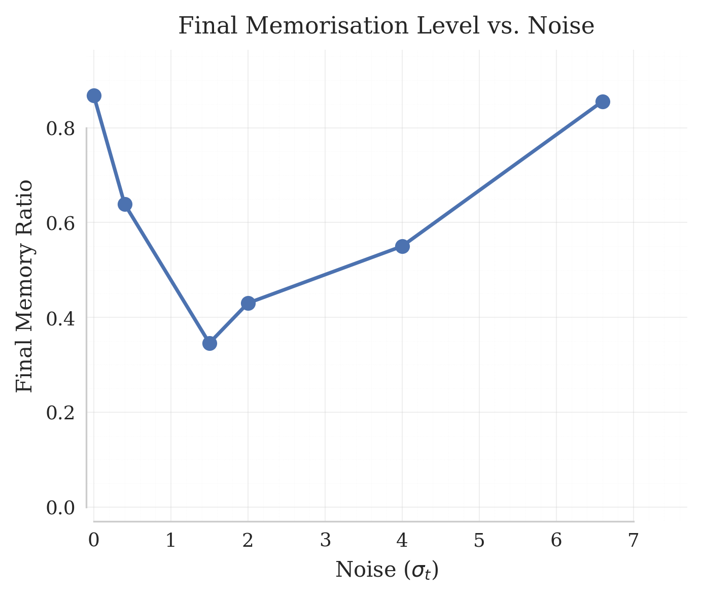
Our main finding is that the crossover location as a function of exhibits the same bell-shaped structure that we observe empirically; suggesting that crossovers remain predictive in the regime governed by algorithm 1. We begin with an empirical study of the affect that algorithm 1 has on memorisation as varies. Figure 1 shows that there is an inverted bell-curve when memorisation ratio is plotted against as when is close to or the trained model exhibits large amounts of memorisation, but for intermediate memorisation is reduced. This suggests that the location of the phase transition from memorisation to generalisation with respect to model capacity would be delayed for intermediate values of .
Now, motivated by the relationship between crossovers and phase transitions in Buchanan et al. (2025) we investigate the properties of the crossovers in the regime of algorithm 1. In fig. 2 we demonstrate that the crossovers exhibit the same bell-shaped dependency on that we observed empirically. We take this as strong evidence that crossovers could be used to accurately predict the affect that has on phase transitions. An exciting prospect for future work is to investigate whether there exists a weight function such that the crossovers predict the location of phase transitions as well as the properties.
(a)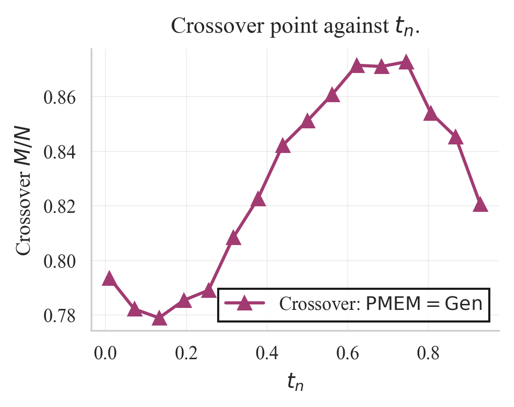
(b)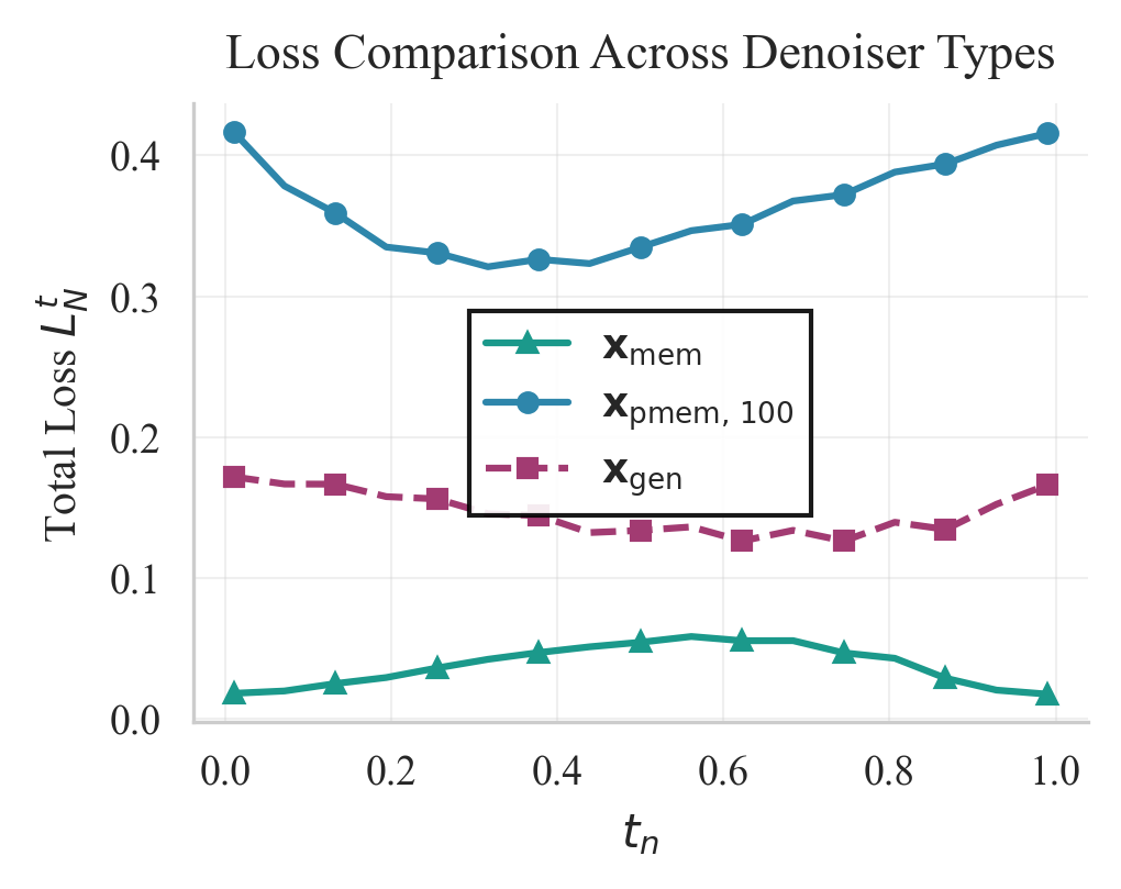
(c)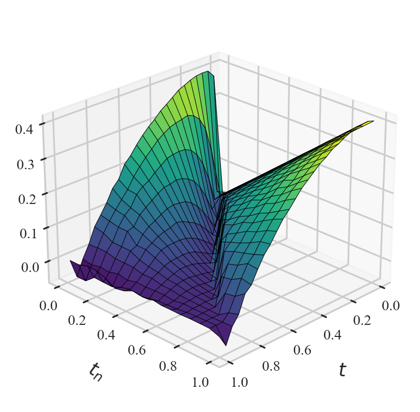
We finish our study under the assumption that loss crossovers predict the locations of phase transition. A notable property of the original crossover theorem 1 is that is linear in . In fig. 3(left) we plot the crossover point as a function of and in the ambient regime and notice limited variation in . This suggests that similar to theorem 1 a crossover occurs when is equal to a fixed constant. Together, all of these results suggest that the loss crossovers retain predictive power over the phase shift even in modified training regimes.
(a)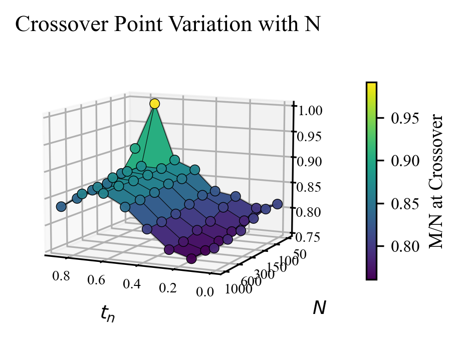
(b)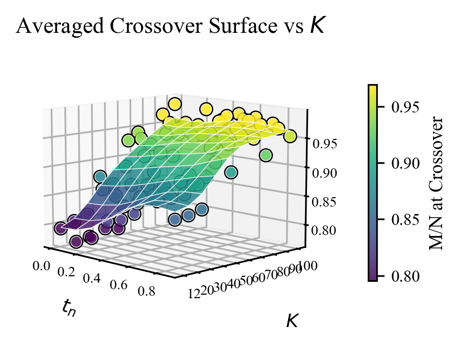
References
- On the edge of memorization in diffusion models. arXiv preprint arXiv:2508.17689. Cited by: §1, §3, §3, Figure 2, §5, Theorem 1.
- Consistent diffusion meets tweedie: training exact ambient diffusion models with noisy data. arXiv preprint arXiv:2404.10177. Cited by: §4.
- On memorization in diffusion models. arXiv preprint arXiv:2310.02664. Cited by: §3, Figure 1.
- Denoising diffusion probabilistic models. Advances in neural information processing systems 33, pp. 6840–6851. Cited by: §2, Figure 1.
- Elucidating the design space of diffusion-based generative models. Advances in neural information processing systems 35, pp. 26565–26577. Cited by: §2.
- Critical windows: non-asymptotic theory for feature emergence in diffusion models. arXiv preprint arXiv:2403.01633. Cited by: §4.
- Least squares estimation without priors or supervision. Neural computation 23 (2), pp. 374–420. Cited by: §2.
- Does generation require memorization? creative diffusion models using ambient diffusion. arXiv preprint arXiv:2502.21278. Cited by: Loss Crossovers and Phase Transitions Under Ambient Training in Diffusion Models, §4, §4, Algorithm 1.
- Score-based generative modeling through stochastic differential equations. arXiv preprint arXiv:2011.13456. Cited by: §2.
- Diffusion models learn low-dimensional distributions via subspace clustering. arXiv preprint arXiv:2409.02426. Cited by: §1, §3.
- The emergence of reproducibility and generalizability in diffusion models. arXiv preprint arXiv:2310.05264. Cited by: §1, §3.